|
Another important geometrical concept associated with a curve leads to
an integration. This is the length of arc. To express the length
analytically by an integral, in fact, we think of the curve as
represented by a function  with a continuous derivative with a continuous derivative  . By
the points . By
the points
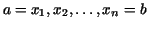 we divide up the interval we divide up the interval
 of the of the  -axis, over which our curve
lies, into -axis, over which our curve
lies, into  subintervals of length subintervals of length
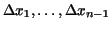 .
In the curve we inscribe a polygon whose vertices lie vertically
above these points. The length of the curve is then defined to be the
limit of the perimeters of these inscribed polygons, provided that
such a limit does exist and is independent of the particular way in
which the polygons are chosen. This assumption is called
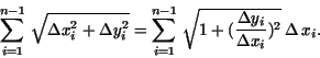
rectifiability. So the total length of the inscribed polygon is given
according to Pythagoras theorem by the expression .
In the curve we inscribe a polygon whose vertices lie vertically
above these points. The length of the curve is then defined to be the
limit of the perimeters of these inscribed polygons, provided that
such a limit does exist and is independent of the particular way in
which the polygons are chosen. This assumption is called
rectifiability. So the total length of the inscribed polygon is given
according to Pythagoras theorem by the expression
But by the mean value theorem of the differential calculus the
difference quotient
 is equal to is equal to  , where , where  is an intermediate value in the interval is an intermediate value in the interval  .
If we now let .
If we now let  increase beyond all bounds and at the same time
let the length of the longest subinterval increase beyond all bounds and at the same time
let the length of the longest subinterval  tend to zero,
then by the definition of integral our expression will tend to the
limit tend to zero,
then by the definition of integral our expression will tend to the
limit
We established the following theorem:
- Theorem 3.
- Every curve
 for which the derivative for which the derivative  is
continuous is a rectifiable curve, and its length between is
continuous is a rectifiable curve, and its length between  and and  (
( ) is given by the formula ) is given by the formula
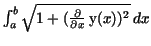 . .
Our expression for the length of arc is still subject to the special
and artifical assumption that the curve consists of one single-valued
branch above the  -axis. Parametric representation frees us from this
restriction. If a curve of the kind which we have been considering is
given in parametric form by the equations -axis. Parametric representation frees us from this
restriction. If a curve of the kind which we have been considering is
given in parametric form by the equations
 , then by
introducing the parameter , then by
introducing the parameter  in the above expression we obtain the
parametric form of the length of arc in the above expression we obtain the
parametric form of the length of arc
where  and and  are the values of are the values of  which correspond respectively to the points of the curve which correspond respectively to the points of the curve  and and  . .
Excercise 7.1. Give the length of the arc when the curve is expressed in
polar coordinates.
EXAMPLE 7.3.
Consider the parabola
 f:=x->1/2*x^2;
For its length of arc we immediately obtain the integral
 Int(sqrt(1+x^2),x=a..b);
which has the value
 value(%);
EXAMPLE 7.4.
As an example for a motion along a path or trajectory consider the
cycloids which arise when a circle rolls along a straight line or
another circle. Here we limit ourselves to the simplest case, in which
a circle of radius  rolls along the rolls along the  -axis, and we consider a point on
its circumference. This point then describes a cycloid. If we choose
the origin of the coordinate system and the initial time in such a way
that for time -axis, and we consider a point on
its circumference. This point then describes a cycloid. If we choose
the origin of the coordinate system and the initial time in such a way
that for time  the corresponding point of the curve coincides with
the origin, we obtain the parametric representation the corresponding point of the curve coincides with
the origin, we obtain the parametric representation
for the cycloid. Here  denotes the angle
through which the circle has turned from its original position. From
the above equations we obtain at once that denotes the angle
through which the circle has turned from its original position. From
the above equations we obtain at once that
Hence the length of the arc is
 Int(sqrt(diff(x(t),t)^2+diff(y(t),t)^2),t=0..alpha)=
 Int(sqrt(2*R^2*(1-cos(t))),t=0..alpha);
Since
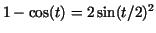 the integrand is equal to the integrand is equal to  , hence for , hence for
 the equation becomes the equation becomes
 Int(2*R*sin(t/2),t=0..alpha);
The value of this integral is
 value(%);
If we consider the length of arc between two successive cusps we must
put
 . Then we have . Then we have
 eval(subs(alpha=2*Pi,%));
Thus, we obtain that the lenght of arc of the cycloid between
successive cusps is equal to four times the diameter of the rolling
circle.
Similarly, we calculate the area bounded by one arch of the cycloid
and the  -axis. If -axis. If  then this area has the form then this area has the form
 plot([t-sin(t),1-cos(t),t=0..2*Pi]);
The area is
 Int(y(t)*diff(x(t),t),t=0..2*Pi)=
 R^2*Int((1-cos(t))^2,t=0..2*Pi);
 value(rhs(%));
This area is therefore three times the area of the rolling circle.
Exercise 7.2. Calculate the area bounded by the semicubical parabola
 , the , the  -axis and the lines -axis and the lines  and and  . Calculate
the length of arc of it. . Calculate
the length of arc of it.
Exercise 7.3. Find the volume and surface area of the torus (or anchor ring) obtained by rotating a circle about a line which does not intersect
it.
Exercise 7.4. Find the area of a catenoid, the surface obtained by
rotating an arc of the catenary  about the about the  -axis. -axis.
The possibilities of applications of differential and integral calculus
are unbounded. In sciences and engineering mathematical models are developed to aid in the understanding of physical phenomena.
These models often yield an equation that contains some derivatives of an unknown function. Such an equation is called differential equation. In order
to solve these equations one requires the theory of integration. In this paper we did the first steps towards better understanding the mathematical and real world in which we live.
| 
![\includegraphics[width=12cm]{int14.ps}](img615.gif)