HEJ, HU ISSN 1418-7108 Manuscript no.: ANM-980205-A

A Circulant Seminorm Representation on the Unit Cube

We give the sparse circulant representation of the $H^{1/2}$ seminorm

$$\mid f \mid^2_{H^{1/2}(\partial U)} = \int_{\partial U} \i... ...\underline y} \Vert^3 } ds({\underline x}) ds({\underline y})$$ (22)

on the boundary $\partial U$ of the unit cube $U$ (1), where $s$ denote the area on $\partial U$ and

$$\Vert{\underline x - \underline y} \Vert = \sqrt{ (x_1 - y_1)^2 + (x_2 - y_2)^2 + (x_3 - y_3)^2}$$ (23)

is the standard euclidean distance in $R^3$.

Let

$$Q_1 = \{ (x,y,z) \mid x=0, \quad 0 \le y \le 1, \quad 0 \le z \le 1 \},$$ (24)

$$Q_2 = \{ (x,y,z) \mid 0 \le x \le 1, \quad y = 0, \quad 0 \le z \le 1 \},$$ (25)

$$Q_3 = \{ (x,y,z) \mid 0 \le x \le 1, \quad 0 \le y \le 1, \quad z = 0 \},$$ (26)

$$Q_4 = \{ (x,y,z) \mid x=1, \quad 0 \le y \le 1, \quad 0 \le z \le 1 \},$$ (27)

$$Q_5 = \{ (x,y,z) \mid 0 \le x \le 1, \quad y = 1, \quad 0 \le z \le 1 \},$$ (28)

$$Q_6 = \{ (x,y,z) \mid 0 \le x \le 1, \quad 0 \le y \le 1, \quad z = 1 \}$$ (29)

denote the sides of $U$ and let $S_i$ $(i=1,2,3)$ denote the strips

$$S_1 = Q_1 \cup Q_2 \cup Q_4 \cup Q_5, \quad$$ (30)

$$S_2 = Q_1 \cup Q_3 \cup Q_4 \cup Q_6, \quad$$ (31)

$$S_3 = Q_2 \cup Q_3 \cup Q_5 \cup Q_6.$$ (32)

In this case the $H^{1/2}$ seminorm on $\partial U$ can be reduced to a sum of 'partial' seminorms as follows:

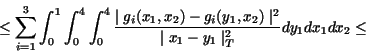
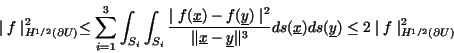
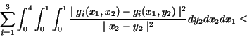
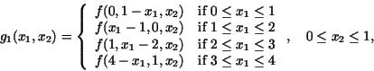
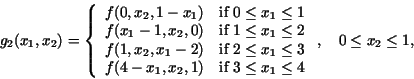
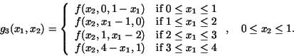
Theorem 4.1   Let $f \in H^{1/2}(\partial U)$. Then

$$2^{-6} \mid f \mid^2_{H^{1/2}(\partial U)} \le$$

$$\le \sum_{i = 1}^{3} \int_0^1 \int_0^4 \int_0^4 \frac{\mi... ..._1,x_2) \mid^2}{ \mid x_1 - y_1 \mid_T^2} dy_1 dx_1 dx_2 \le$$ (33)

$$\le 2^{7} \mid f \mid^2_{H^{1/2}(\partial U)}.$$

where

$$\mid x_1 - y_1 \mid_T = \min \{ \mid x_1 - y_1 \mid, 4 - \mid x_1 - y_1 \mid \}$$ (34)

and the functions $g_i$ $(i=1,2,3)$ are defined as follows:

$$g_1(x_1,x_2) = \left\{ \begin{array}{ll} f(0, 1-x_1, x_2)... ...x_1 \le 4 $}\\ \end{array} \right. , \quad 0 \le x_2 \le 1,$$ (35)

$$g_2(x_1,x_2) = \left\{ \begin{array}{ll} f(0, x_2, 1-x_1 ... ...x_1 \le 4$} \\ \end{array} \right. , \quad 0 \le x_2 \le 1,$$ (36)

$$g_3(x_1,x_2) = \left\{ \begin{array}{ll} f(x_2, 0, 1-x_1 ... ...x_1 \le 4$} \\ \end{array} \right. , \quad 0 \le x_2 \le 1.$$ (37)

Proof 4.2   A simple calculation gives

$$\mid f \mid^2_{H^{1/2}(\partial U)} \le \sum_{i=1}^{3} \... ...ds({\underline y}) \le 2 \mid f \mid^2_{H^{1/2}(\partial U)}$$ (38)

and

$$2^{-2} \int_{S_i} \int_{S_i} \frac{\mid f({\underline x}) ... ...rline y} \Vert^3 } ds({\underline x}) ds({\underline y}) \le$$

$$\le \int_0^4 \int_0^1 \int_0^4 \int_0^1 \frac{\mid g_i(x_... ...T^2 + \mid x_2 - y_2 \mid^2 )^{3/2}} dy_2 dy_1 dx_2 dx_1 \le$$ (39)

$$\le 2^{3/2} \int_{S_i} \int_{S_i} \frac{\mid f({\underlin... ...t^3 } ds({\underline x}) ds({\underline y}), \quad (i=1,2,3).$$

Theorem 2.1 implies that

$$2^{-5} \int_0^4 \int_0^1 \int_0^4 \int_0^1 \frac{\mid g_i... ...T^2 + \mid x_2 - y_2 \mid^2 )^{3/2}} dy_2 dy_1 dx_2 dx_1 \le$$

$$\le \int_0^4 \int_0^1 \int_0^1 \frac{\mid g_i(x_1,x_2) - g_i(x_1,y_2) \mid^2} { \mid x_2 - y_2 \mid^2} dy_2 dx_2 dx_1 +$$ (40)

$$+ \int_0^1 \int_0^4 \int_0^4 \frac{\mid g_i(x_1,x_2) - g_i(y_1,x_2) \mid^2} {\mid x_1 - y_1 \mid_T^2} dy_1 dx_1 dx_2 \le$$

$$\le 2^{4} \int_0^4 \int_0^1 \int_0^4 \int_0^1 \frac{\mid ... ...2 - y_2 \mid^2 )^{3/2}} dy_2 dy_1 dx_2 dx_1, \quad (i=1,2,3).$$

Since

$$\sum_{i=1}^{3} \int_0^4 \int_0^1 \int_0^1 \frac{\mid g_i(... ...x_1,y_2) \mid^2} { \mid x_2 - y_2 \mid^2} dy_2 dx_2 dx_1 \le$$ (41)

$$\le 2 \sum_{i=1}^{3} \int_0^1 \int_0^4 \int_0^4 \frac{\m... ..._i(y_1,x_2) \mid^2} {\mid x_1 - y_1 \mid_T^2} dy_1 dx_1 dx_2$$

summing up the inequalities (38)-(41) the proof is completed.

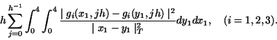
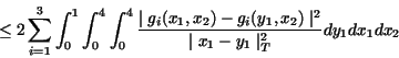
Assume that $\partial U$ is endowed with a uniform square mesh with a grid size $h$ and $V_h(\partial U)$ denotes the space of piecewise bilinear finite elements corresponding to this discretization. Then if $f \in V_h(\partial U)$ we can apply Theorem 3.1 for the functions $g_i$ $(i=1,2,3)$ in Theorem 4.1. and so the 'partial' seminorms

$$\int_0^1 \int_0^4 \int_0^4 \frac{\mid g_i(x_1,x_2) - g_i(y... ...^2}{ \mid x_1 - y_1 \mid_T^2} dy_1 dx_1 dx_2, \quad (i=1,2,3)$$ (42)

can be substituted by the following sum of the one-dimensional circulant seminorms:

$$h\sum_{j=0}^{h^{-1}} \int_0^4 \int_0^4 \frac{\mid g_i(x_1,... ...\mid^2}{ \mid x_1 - y_1 \mid_T^2} dy_1 dx_1, \quad (i=1,2,3).$$ (43)

Hence using the sparse circulant matrix representation [6] of the one-dimensional seminorm $H^{1/2}$ we can give a sparse matrix representation of the $H^{1/2}$ seminorm in $V_h(\partial U)$ which contains $O(Nlog(N))$ non-zero elements, where $N$ is the number of the unknowns.

Remark 4.3   It is easy to see that the construction given above makes possible the application of the two-dimensional $BPS$ [1] preconditioner to three-dimensional problems. In such a way we get a wire basket type preconditioner $P_{BPS}$ for wich the estimate

$$\alpha_1 (P_{BPS} \underline f, \underline f) \le$$

$$\le \sum_{i = 1}^{3} \int_0^1 \int_0^4 \int_0^4 \frac{\mi... ..._1,x_2) \mid^2}{ \mid x_1 - y_1 \mid_T^2} dy_1 dx_1 dx_2 \le$$ (44)

$$\le \alpha_2 (P_{BPS} \underline f, \underline f)$$

holds, where $\frac{\alpha_2}{\alpha_1} \le C(1+(log(h^{-1}))^2)$ and $C$ is a positive constant independent from the mesh size $h$.

HEJ, HU ISSN 1418-7108 Manuscript no.: ANM-980205-A