HEJ, HU ISSN 1418-7108
Manuscript no.: ANM-981030-A
| 

 |
|
Let us first recall the principal equations.
We get from the Maxwell equations in the magnetostatic case
the relations
with
 in the nonlinear model, cf. [8].
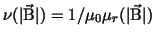
Here, the magnetic field strength is denoted by
in the nonlinear model, cf. [8].
Here, the magnetic field strength is denoted by
 ,
the magnetic induction by ,
the magnetic induction by
 , and , and
 is the current density.
Since (3)
holds, we can introduce the magnetic vector potential
is the current density.
Since (3)
holds, we can introduce the magnetic vector potential
 by
by
 |
(4) |
In magnetostatics, the Coulomb gauge
 |
(5) |
is standard.
Thus, we end up with the equations
for the unknown vector potential
.
If permanent magnets are involved,
must be replaced by
 .
According to material properties, the coefficient .
According to material properties, the coefficient  depends on the position
  .
With the unknown .
With the unknown
 , equations (6) and (7)
can be rewritten as , equations (6) and (7)
can be rewritten as
We can formulate a linear problem by the equations
(10) and (9),
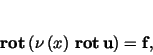 |
(10) |
which is a good approximation for the nonlinear problem
if we can neglect saturation effects in ferromagnetic materials.
| HEJ, HU ISSN 1418-7108
Manuscript no.: ANM-981030-A
|
|
|