HEJ, HU ISSN 1418-7108 Manuscript no.: ANM-981030-A

   
Spaces

In the following, we always assume that $\Gamma=\partial\Omega$ and all interfaces between different materials are sufficiently smooth (e.g. piecewise from $C^2$). We use the standard Sobolev spaces (cf. e.g., [7]) $L^2(\Omega)$ and $L^2(\Omega)^3$ equipped with the norm $\vert\vert.\vert\vert _0$ and the scalar product $(.,.)_0$, and the space

$$L^2_\star(\Omega) = \left\{ \lambda \in L^2(\Omega) : (\lambda,1)_0 = \int_\Omega \lambda \; dx = 0 \right\}.$$

Next, we define the space $H^1(\Omega)^3$ with

$$\vert{\bf v}\vert _1^2 = \vert\vert { \bf grad }{\bf v} \vert\vert _0^2 = \int_\Omega {\bf v}_{i,j} {\bf v}_{i,j} \;dx,$$

where ${\bf v}_{i,j} = \frac{\partial {\bf v}_i}{\partial x_j}$ and Einstein's summation convention is applied to indices $i$ and $j$, and

$$\vert\vert{\bf v}\vert\vert _1^2 = \vert{\bf v}\vert _1^2 + \vert\vert{\bf v}\vert\vert _0^2.$$

It is a standard result that $\vert.\vert _1$ is a norm of $H^1_0(\Omega)^3$. The following lemma (cf. [6]) allows us to represent the norm $\vert.\vert _1$ of the $H^1_0(\Omega)^3$.

Lemma 1   For all ${\bf v}\in H^1_0(\Omega)^3$ the equation

$$\vert{\bf v}\vert _1^2 = \vert\vert{ \bf rot }{\bf v}\vert\vert _0^2 + \vert\vert\div {\bf v}\vert\vert _0^2$$ (16)

holds.

Proof. Assume ${\bf v}\in H^2(\Omega)^3$. We rewrite the ${ \bf rot }\;$ operator as follows

$$\begin{eqnarray*} \int_\Omega { \bf rot }{\bf v} \cdot { \bf rot }{\bf v} \... ...t_\Omega {\bf v}_{i,j} {\bf v}_{i,j} - (\div {\bf v})^2 \;dx, \end{eqnarray*}$$

and after having applied partial integration twice we arrive at

$$\vert\vert{ \bf rot }{\bf v}\vert\vert _0^2 = \vert{\bf v... ...quad \forall {\bf v}\in H^1_0(\Omega)^3 \cap H^2(\Omega)^3.$$ (17)

Since $H^1_0(\Omega)^3 \cap H^2(\Omega)^3$ is dense in $H^1_0(\Omega)^3$, equation (16) holds for all ${\bf v}\in H^1_0(\Omega)^3$.
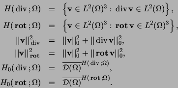
Let us discuss further spaces, cf. [4]. We define

$$\begin{eqnarray*} H(\div ;\Omega) &=& \left\{{\bf v}\in L^2(\Omega)^3 : \div {\... ...ega) &=& \overline{{\cal D}(\Omega)}^{H({ \bf rot };\Omega)}. \end{eqnarray*}$$

It is proved in [7] that

$$H^1_0(\Omega)^3 = H_0(\div ;\Omega) \cap H_0({ \bf rot };\Omega).$$

We remark that $H_0(\div ;\Omega)$ has a zero trace of the normal component on $\Gamma=\partial\Omega$, whereas $H_0({ \bf rot };\Omega)$ has a zero trace of the tangential component. Therefore, the space $H_0({ \bf rot };\Omega)$ seems to be appropriate to the flux line boundary condition, cf. (12). Since we are interested in formulating a gauge condition that involves the divergence of the vector potential, we introduce the space

$${\bf Y}= H_0({ \bf rot };\Omega) \cap H(\div ;\Omega)$$ (18)

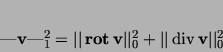
equipped with the norm

$$\vert\vert{\bf v}\vert\vert _{\bf Y}^2 = \vert\vert{\bf v... ...f v}\vert\vert _0^2 + \vert\vert\div {\bf v}\vert\vert _0^2.$$ (19)

>From [7], we have the following results.

Lemma 2   Assume that $\Omega$ is bounded, Lipschitz-continuous, simply-connected and $\Gamma$ has just one component. Then there exists a positive constant $c$ such that

$$\vert\vert{\bf v}\vert\vert _0 \le c \left( \vert\vert{ \b... ...f v}\vert\vert _0 \right) \quad \forall {\bf v} \in {\bf Y}$$

holds.

Proof. See [7], Lemma 3.4.

Lemma 3   Assume that $\Omega$ is bounded, Lipschitz-continuous, simply-connected and $\Gamma$ has just one component. Then, the seminorm

$$\vert{\bf v}\vert _{\bf Y}= \left( \vert\vert{ \bf rot ... ...rt _0^2 + \vert\vert\div {\bf v}\vert\vert _0^2 \right)^{1/2}$$ (20)

is a norm in Y, too.

Proof. Lemma 3 is a direct consequence of Lemma 2.
The next lemma requires more than the standard assumptions for technical magnetic field problems. Indeed, electromagnetic devices may have re-entrant corners. Therefore, we will not base our further investigations on Lemma 4.

Lemma 4   Assume further that either $\Omega$ has a ${\cal C}^{1,1}$ boundary, or $\Omega$ is a convex polyhedron. Then ${\bf Y}$ is continuously imbedded in $H^1(\Omega)^3$.

Proof. See [7], Theorem 3.7.

HEJ, HU ISSN 1418-7108 Manuscript no.: ANM-981030-A