HEJ, HU ISSN 1418-7108
Manuscript no.: ANM-981030-A
| 

 |
|
Equivalence with magnetostatics
Next, we have to prove that the solution
 of the variational problem (23), (24)
represents a solution of the magnetostatic problem, too.
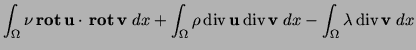
Indeed, in (23) we have added the terms
of the variational problem (23), (24)
represents a solution of the magnetostatic problem, too.
Indeed, in (23) we have added the terms
 and
and
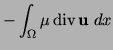
 to the formulation of (15).
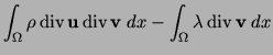
We show that for the solution
the sum of both terms vanishes.
We recall the following theorem from [7].
to the formulation of (15).
We show that for the solution
the sum of both terms vanishes.
We recall the following theorem from [7].
THEOREM 3
Assume that  is bounded, Lipschitz-continuous and simply-connected.
A function
 satisfies
iff there exists a unique function
such that
Proof. See [7], Theorem 2.9.
In the next theorem, we will assume that the electrical current density
 is divergence-free.
Indeed, since electrical charges cannot appear or disappear,
this assumption represents the physical behaviour. is divergence-free.
Indeed, since electrical charges cannot appear or disappear,
this assumption represents the physical behaviour.
THEOREM 4
Assume that is bounded, Lipschitz-continuous and simply-connected.
Assume further that
 is divergence-free,
i.e.,
 |
(34) |
Then, the unique solution
of
fulfills
 |
(37) |
Proof.
Let us choose an arbitrary
 .
Then it is well-known that the Dirichlet problem .
Then it is well-known that the Dirichlet problem
has a unique weak solution
 .
>From Theorem 3 we deduce that there exists a
with .
>From Theorem 3 we deduce that there exists a
with
 |
(40) |
and
 |
(41) |
Next, from (39) we get that the tangential derivatives
of  vanish, i.e. that the tangential components of vanish, i.e. that the tangential components of  are zero.
Thus,
are zero.
Thus,
 holds.
Further, we can determine the divergence of as follows holds.
Further, we can determine the divergence of as follows
Consequently,
 and and
 .
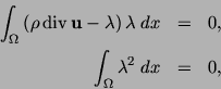
We can apply as a test function in
(35), and we get with (40) .
We can apply as a test function in
(35), and we get with (40)
With the assumptions
(39) and (34) on and ,
the right-hand side is zero.
Therefore,
 |
(46) |
holds, and setting
 for any
, we arrive at (37).
for any
, we arrive at (37).
Thus, with (15) we get
 |
(47) |
and we conclude the relation
 |
(48) |
in the weak sense.
We remark that we do not require that
 on on
 .
Further,
setting .
Further,
setting
 ,
we get from (46) and (36) that ,
we get from (46) and (36) that
and  . Therefore, we can omit the . Therefore, we can omit the  -term in
(35), and solve the coercive problem: -term in
(35), and solve the coercive problem:
(VF1 ) Find ) Find
 such that
 |
(49) |
The unique solution  of (VF1) coincides with the
in the solution of (VF1). We may discretize and solve the problem in the
formulation (VF1) instead of (VF1). of (VF1) coincides with the
in the solution of (VF1). We may discretize and solve the problem in the
formulation (VF1) instead of (VF1).
| HEJ, HU ISSN 1418-7108
Manuscript no.: ANM-981030-A
|
|
|